floodlight.models.geometry

class floodlight.models.geometry.CentroidModel

Computations based on the geometric center of all players, commonly referred to as a team’s centroid.

Upon calling the fit()-method, this model calculates a team’s centroid. The following calculations can subsequently be queried by calling the corresponding methods:

• Centroid [1] –> centroid()

• Centroid Distance –> centroid_distance()

• Stretch Index [2] –> stretch_index()

Notes

Team centroids are computed as the arithmetic mean of all player positions (based on numpy’s nanmean function). For a fixed point in time and \(N\) players with corresponding positions \(x_1, \dots, x_N \in \mathbb{R}^2\), the centroid is calculated as

\[C = \frac{1}{N} \sum_i^N x_i.\]

Examples

>>> import numpy as np
>>> from floodlight import XY
>>> from floodlight.models.geometry import CentroidModel

>>> xy = XY(np.array(((1, 1, 2, -2), (1.5, np.nan, np.nan, -0))))
>>> cm = CentroidModel()
>>> cm.fit(xy)
>>> cm.centroid()
XY(xy=array([[ 1.5, -0.5],
   [ 1.5,  0. ]]), framerate=None, direction=None)
>>> cm.stretch_index(xy)
TeamProperty(property=array([1.5811388, nan]), name='stretch_index', framerate=None)
>>> cm.stretch_index(xy, axis='x')
TeamProperty(property=array([0.5, 0.]), name='stretch_index', framerate=None)

References

[1]

Sampaio, J., & Maçãs, V. (2012). Measuring tactical behaviour in football. International Journal of Sports Medicine, 33(05), 395-401.

[2]

Bourbousson, J., Sève, C., & McGarry, T. (2010). Space–time coordination dynamics in basketball: Part 2. The interaction between the two teams. Journal of Sports Sciences, 28(3), 349-358.

centroid()

Returns the team centroid positions as computed by the fit method.

Returns:

centroid – An XY object of shape (T, 2), where T is the total number of frames. The two columns contain the centroids’ x- and y-coordinates, respectively.

Return type:

XY

centroid_distance(xy, axis=None)

Calculates the Euclidean distance of each player to the fitted centroids.

Parameters:

• xy (XY) – Player spatiotemporal data for which the distances to the fitted centroids are calculated.

• axis ({None, ‘x’, ‘y’}, optional) – Optional argument that restricts distance calculation to either the x- or y-dimension of the data. If set to None (default), distances are calculated in both dimensions.

Returns:

centroid_distance – A PlayerProperty object of shape (T, N), where T is the total number of frames. Each column contains the distances to the team centroid of the player with corresponding xID.

Return type:

PlayerProperty

fit(xy, exclude_xIDs=None)

Fit the model to the given data and calculate team centroids.

Parameters:

• xy (XY) – Player spatiotemporal data for which the centroid is calculated.

• exclude_xIDs (list, optional) – A list of xIDs to be excluded from computation. This can be useful if one would like, for example, to exclude goalkeepers from analysis.

stretch_index(xy, axis=None)

Calculates the Stretch Index, i.e., the mean distance of all players to the team centroid.

Parameters:

• xy (XY) – Player spatiotemporal data for which the stretch index is calculated.

• axis ({None, ‘x’, ‘y’}, optional) – Optional argument that restricts stretch index calculation to either the x- or y-dimension of the data. If set to None (default), the stretch index is calculated in both dimensions.

Returns:

stretch_index – A TeamProperty object of shape (T,), where T is the total number of frames. Each entry contains the stretch index of that particular frame.

Return type:

TeamProperty

class floodlight.models.geometry.ConvexHullModel

Computations based on the convex hull of player positions.

Upon calling the fit() method, this model calculates convex hull objects for each frame. The following calculations can subsequently be queried by calling the corresponding methods:

• Convex Hull Area –> convex_hull_area()

• Convex Hull Visualization –> plot()

Notes

The convex hull is computed using scipy’s ConvexHull class and can be understood as the minimal convex area containing all (outfield) players.

The convex hull is also known in the literature under the terms ‘surface area’, ‘coverage area’ and ‘playing area’ [3].

When multiple XY objects are provided, all players from all teams are combined and the convex hull encompasses all of them. This is commonly referred to as the Effective Area of Play (EAP) [4].

Examples

>>> import numpy as np
>>> from floodlight import XY
>>> from floodlight.models.geometry import ConvexHullModel

Single team convex hull (excluding goalkeeper):

>>> xy = XY(np.array([[0, 0, 10, 0, 10, 10, 0, 10],
...                   [0, 0, 10, 0,  5, 10, 5,  5]]))
>>> chm = ConvexHullModel()
>>> chm.fit(xy, exclude_xIDs=[[0]])
>>> chull = chm.convex_hull_area()
>>> chull
TeamProperty(property=array([50., 12.5]), name='convex_hull_area', framerate=None)

Effective Area of Play (both teams):

>>> xy_home = XY(np.array([[0, 10, 20, 20], [10, 20, 10, 20]]))
>>> xy_away = XY(np.array([[40, 50, 60, 60], [50, 70, 50, 60]]))
>>> chm = ConvexHullModel()
>>> chm.fit([xy_home, xy_away])
>>> eap = chm.convex_hull_area()
>>> eap
TeamProperty(property=array([400., 200.]), name='convex_hull_area', framerate=None)

References

[3]

Moura, F. A., Martins, L. E. B., Anido, R. D. O., De Barros, R. M. L., & Cunha, S. A. (2012). Quantitative analysis of Brazilian football players’ organisation on the pitch. Sports biomechanics, 11(1), 85-96.

[4]

Clemente, M. F., Couceiro, S. M., Martins, F. M., Mendes, R., & Figueiredo, A. J. (2013). Measuring Collective Behaviour in Football Teams: Inspecting the impact of each half of the match on ball possession. International Journal of Performance Analysis in Sport, 13(3), 678-689.

convex_hull_area()

Calculates the area enclosed by the convex hull.

Returns:

convex_hull_area – A TeamProperty object of shape (T,), where T is the total number of frames. Each entry contains the area enclosed by the convex hull for that frame. Frames with insufficient valid points have NaN values.

Return type:

TeamProperty

Notes

If the model was fitted with:

• Single XY object: returns the team’s convex hull area

• Multiple XY objects: returns the effective area of play (EAP)

fit(xy, exclude_xIDs=None)

Fit the model to the given data and calculate convex hulls.

Parameters:

• xy (XY or list[XY]) – Single XY object or list of XY objects. If list, all XY objects will be combined and the convex hull will encompass all players (effective playing space).

• exclude_xIDs (list[list], optional) – For each XY object, a list of xIDs to exclude from computation. This can be useful to exclude goalkeepers from analysis. Length must match number of XY objects.

  Examples:

  • Single XY with xID=0 excluded: [[0]]

  • Two XYs with both xID=0 excluded: [[0], [0]]

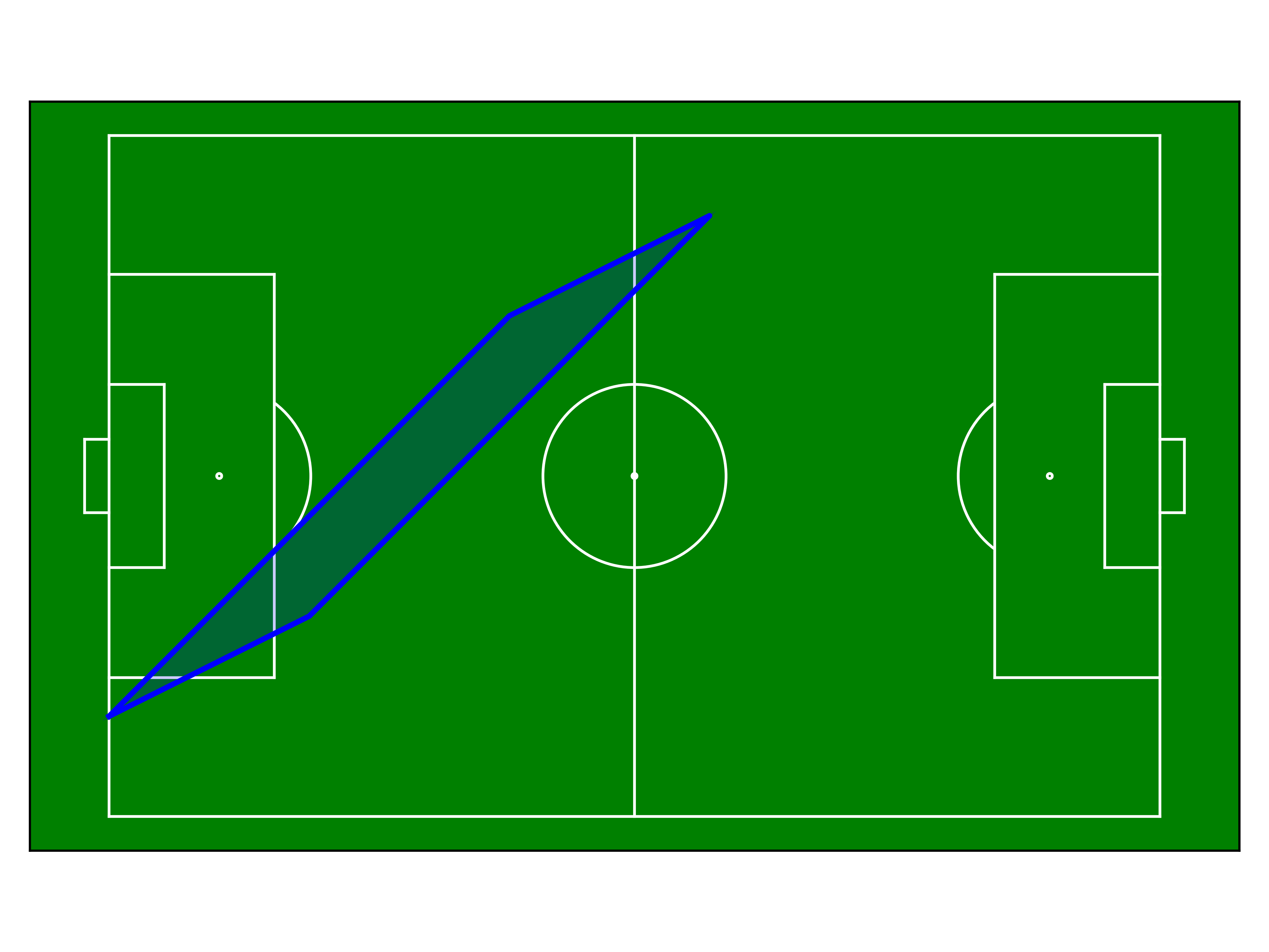
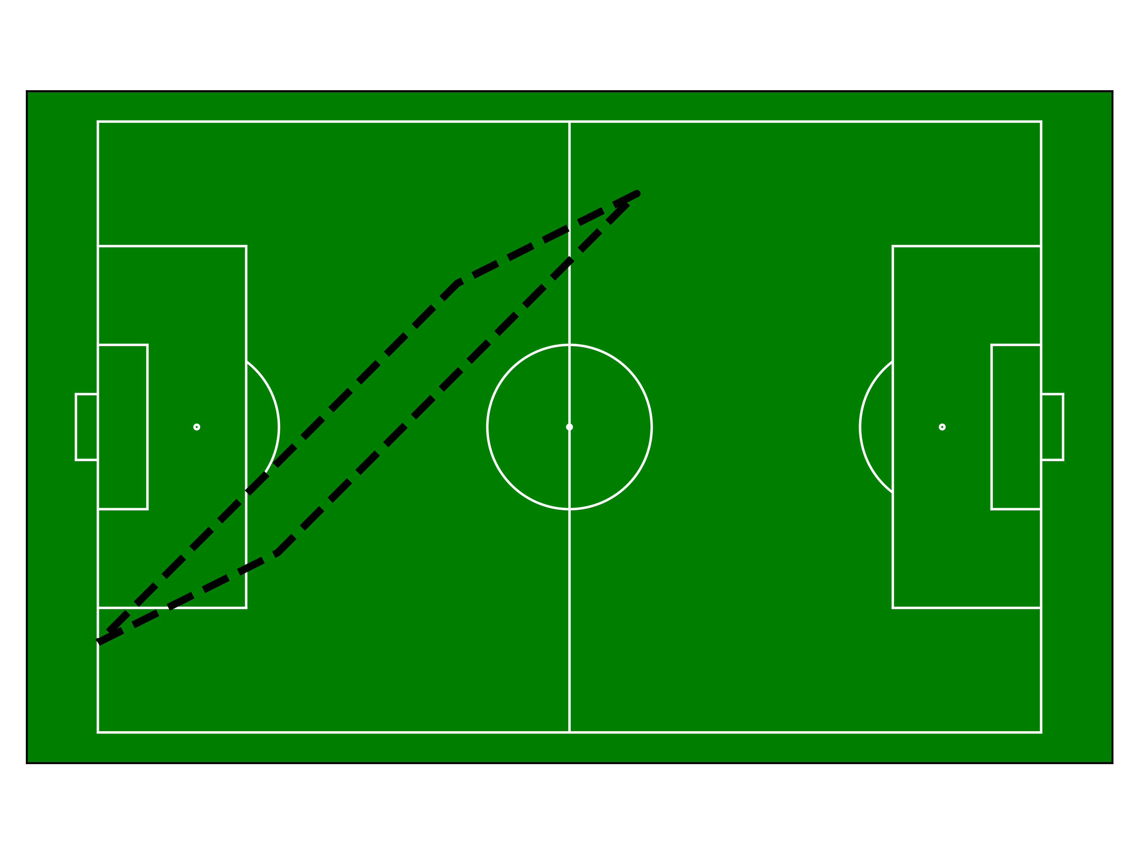
plot(t, ax=None, fill=True, fill_alpha=0.3, **kwargs)

Plot the convex hull for a given time point on a matplotlib axes.

Parameters:

• t (int) – Frame index to plot.

• ax (matplotlib.axes.Axes, optional) – Matplotlib axes to plot on. If None, a new figure and axes are created.

• fill (bool, optional) – Whether to fill the convex hull polygon. Default is True.

• fill_alpha (float, optional) – Transparency of the fill (0=transparent, 1=opaque). Default is 0.3. Only used if fill=True.

• **kwargs (optional) – Additional keyword arguments passed to the line plot. Common options:

  • color : str, default ‘black’

  • alpha : float, default 1.0 (line transparency)

  • linewidth : float, default 2

  • linestyle : str (e.g., ‘–’, ‘:’)

  • Any other matplotlib.axes.Axes.plot() parameters

Returns:

ax – The axes object with the convex hull plotted.

Return type:

matplotlib.axes.Axes

Notes

The kwargs are passed to the plot function of matplotlib for drawing the hull boundary. To customize the plots have a look at matplotlib.

Examples

>>> import matplotlib.pyplot as plt
>>> from floodlight import Pitch
>>>
>>> pitch = Pitch(
... xlim=(0, 105), ylim=(0, 68), sport="football", unit="m", boundaries="fixed"
... )
>>>
>>> fig, ax = plt.subplots()
>>> pitch.plot(ax=ax)
>>>
>>> # Filled hull with custom color
>>> chm.plot(t=0, ax=ax, color='blue', fill_alpha=0.2)

>>> # Dashed outline, no fill
>>> chm.plot(t=0, ax=ax, fill=False, linestyle="--", linewidth=3)

class floodlight.models.geometry.NearestMateModel

Computations for within-team distance metrics.

Upon calling the fit()-method, this model calculates pairwise distances between all players for each frame. The following calculations can subsequently be queried by calling the corresponding methods:

• Distance to Nearest Mate –> distance_to_nearest_mate()

• Team Spread [5] –> team_spread()

Notes

The calculations are performed as follows:

• Distance to Nearest Mate (DTNM):

  For each player in each frame, the Euclidean distance to their nearest teammate is computed.

• Team Spread:

  The Frobenius norm of the lower triangular matrix of all pairwise player distances, representing the overall dispersion of the team.

Examples

>>> import numpy as np
>>> from floodlight import XY
>>> from floodlight.models.geometry import NearestMateModel

>>> xy = XY(np.array(((1, 1, 2, -2), (1.5, np.nan, np.nan, -0))))
>>> nmm = NearestMateModel()
>>> nmm.fit(xy)

>>> dtnm = nmm.distance_to_nearest_mate()
>>> dtnm
PlayerProperty(property=array([[3.16227766, 3.16227766],
       [nan, nan]]), name='distance_to_nearest_mate', framerate=None)
>>> dtnm.property.mean(axis=1)  # Mean distance per frame
array([3.16227766, nan])

>>> nmm.team_spread()
TeamProperty(property=array([3.16227766, nan]), name='team_spread', framerate=None)

References

[5]

Bartlett, R., Button, C., Robins, M., Dutt-Mazumder, A., & Kennedy, G. (2012). Analysing team coordination patterns from player movement trajectories in soccer: Methodological considerations. International Journal of Performance Analysis in Sport, 12(2), 398-424.

distance_to_nearest_mate()

Calculates the distance to the nearest teammate for each player.

Returns:

distance_to_nearest_mate – A PlayerProperty object of shape (T, N), where T is the total number of frames and N is the number of players. Each entry contains the distance to the nearest teammate for that player in that frame.

Return type:

PlayerProperty

fit(xy)

Fit the model to the given data and calculate pairwise distances.

Parameters:

xy (XY) – Player spatiotemporal data for which the pairwise distances are calculated.

team_spread()

Calculates the team spread (Frobenius norm of distance matrix).

Returns:

spread – A TeamProperty object of shape (T,), where T is the total number of frames. Each entry contains the team spread (Frobenius norm of the pairwise distance matrix) for that frame.

Return type:

TeamProperty

class floodlight.models.geometry.NearestOpponentModel

Computations for between-team distance metrics.

Upon calling the fit()-method, this model calculates pairwise distances between players of opposing teams. The following calculations can subsequently be queried:

• Distance to Nearest Opponent [6] –> distance_to_nearest_opponent()

Notes

For each player in each frame, the Euclidean distance to their nearest opponent is computed.

References

[6]

Gonçalves, B., Marcelino, R., Torres-Ronda, L., Torrents, C., & Sampaio, J. (2016). Effects of emphasising opposition and cooperation on collective movement behaviour during football small-sided games. Journal of sports sciences, 34(14), 1346-1354.

Examples

>>> import numpy as np
>>> from floodlight import XY
>>> from floodlight.models.geometry import NearestOpponentModel

>>> xy1 = XY(np.array(((1, 1, 2, -2), (1.5, np.nan, np.nan, -0))))
>>> xy2 = XY(np.array(((2, 2, -1, -1), (0.5, np.nan, np.nan, 1))))
>>> nom = NearestOpponentModel()
>>> nom.fit(xy1, xy2)

>>> dtno1, dtno2 = nom.distance_to_nearest_opponent()
>>> dtno1
PlayerProperty(property=array([[1.41421356, 3.16227766],
       [nan, nan]]), name='distance_to_nearest_opponent', framerate=None)
>>> dtno1.property.mean(axis=1)  # Mean distance per frame
array([2.28824561, nan])

distance_to_nearest_opponent()

Calculates distance to nearest opponent for each player on both teams.

Returns:

distance_to_nearest_opponent – A tuple of two PlayerProperty objects of shape (T, N) containing distances to nearest opponent for each player in the first and second team for each frame.

Return type:

tuple[PlayerProperty, PlayerProperty]

fit(xy1, xy2)

Fit the model to the given data and calculate pairwise distances.

Parameters:

• xy1 (XY) – Player spatiotemporal data for the first team.

• xy2 (XY) – Player spatiotemporal data for the second team.