floodlight.transforms.filter

floodlight.transforms.filter.butterworth_lowpass(xy, order=3, Wn=1, remove_short_seqs=False, **kwargs)

Applies a digital Butterworth lowpass-filter to an XY data object. [1]

For filtering, the scipy.filter.butter and the scipy.signal.filtfilt functions are used. This function provides a convenience access to both functions, directly applying the filter to all non-NaN sequences in all columns.

Parameters:

• xy (XY) – Floodlight XY Data object.

• order (int, optional) – The order of the filter. Corresponds to the argument N from the scipy. signal.butter function. Default is 3

• Wn (Numeric, optional) – The normalized critical cutoff frequency. Corresponds to the argument Wn from the scipy.signal.butter function. Default is 1.

• remove_short_seqs (bool, optional) – If True, sequences that are too short for the filter with the specified settings are replaced with np.nan. If False, they are kept unfiltered. Default is False.

• kwargs – Optional arguments {‘padtype’, ‘padlen’, ‘method’, ‘irlen’} that can be passed to the scipy.signal.filtfilt function.

Returns:

xy_filtered – XY object with position data filtered by designed Butterworth low pass filter.

Return type:

XY

Notes

The values of the input data are assumed to be numerical. Missing data is assumed to be either np.nan or None. The Butterworth-filter requires a minimum signal length depending on the settings. A signal is a sequence of data in the XY-object that is not interrupted by missing values. The minimum signal length is defined as \(3 \cdot (order + 1)\). The treatment of signals shorter than the minimum signal length are specified with the remove_short_sequence-argument, where True will replace these sequences with np.nan and False will keep the sequences in the data unfiltered.

Examples

>>> import numpy as np
>>> import matplotlib.pyplot as plt
>>> from floodlight import XY
>>> from floodlight.transforms.filter import butterworth_lowpass

We first generate a noisy XY-object to smooth.

>>> t = np.linspace(-5, 5, 1000)
>>> player_x = np.sin(t) * t + np.random.rand(1000)
>>> player_x[450:495] = np.nan
>>> player_x[505:550] = np.nan
>>> player_y = t + np.random.randn()
>>> xy = XY(np.transpose(np.stack((player_x, player_y))), framerate=20)

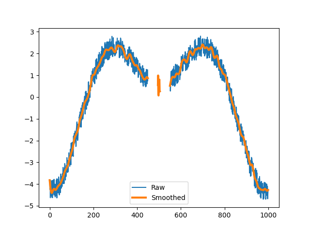
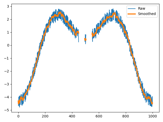
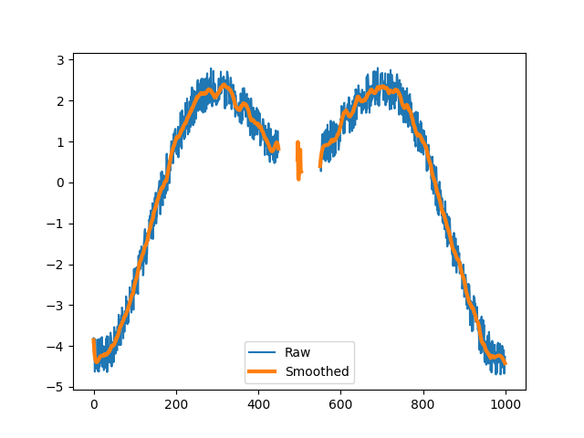
Apply the Butterworth lowpass filter with its default settings.

>>> xy_filt = butterworth_lowpass(xy)
>>> plt.plot(xy.x)
>>> plt.plot(xy_filt.x, linewidth=3)
>>> plt.legend(("Raw", "Smoothed"))
>>> plt.show()

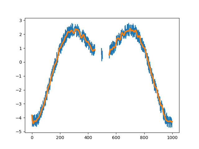
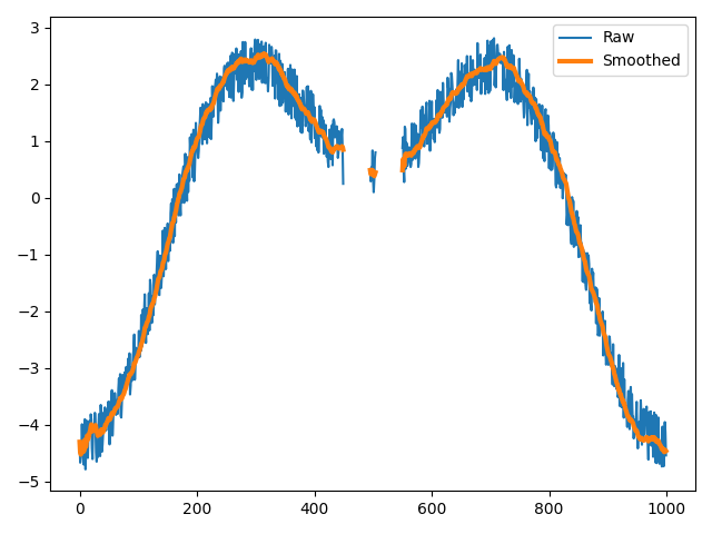
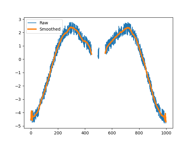
Apply the same filter but remove the sequence that is too short to filter.

>>> xy_filt = butterworth_lowpass(xy, remove_short_seqs=True)
>>> plt.plot(xy.x)
>>> plt.plot(xy_filt.x, linewidth=3)
>>> plt.legend(("Raw", "Smoothed"))
>>> plt.show()

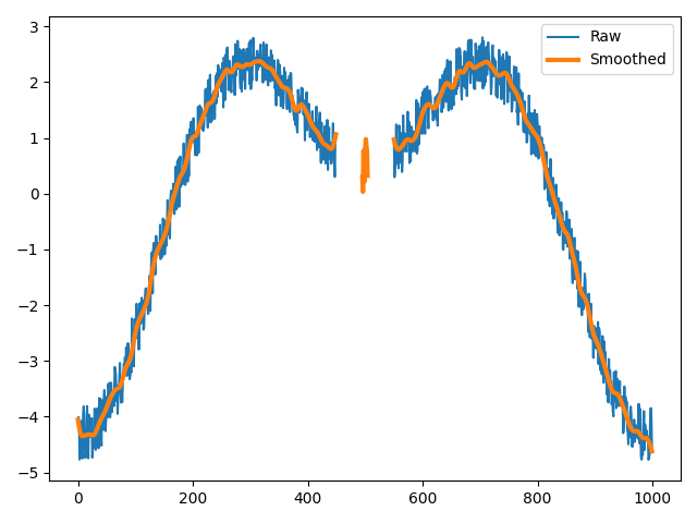
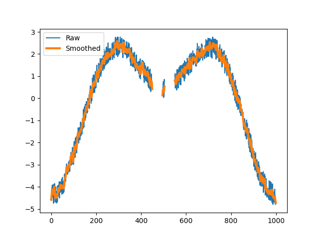
Apply the filter with different specifications.

>>> xy_filt = butterworth_lowpass(xy, order=5, Wn=4)
>>> plt.plot(xy.x)
>>> plt.plot(xy_filt.x, linewidth=3)
>>> plt.legend(("Raw", "Smoothed"))
>>> plt.show()

References

[1]

Butterworth, S. (1930). On the theory of filter amplifiers. Wireless Engineer, 3, 536-541.

floodlight.transforms.filter.fir_lowpass(xy, numtaps=21, cutoff=1, window='hamming', remove_short_seqs=False, **kwargs)

Applies a FIR lowpass-filter to an XY data object.

For filtering, the scipy.signal.firwin and the scipy.signal.filtfilt functions are used. This function provides a convenience access to both functions, directly applying the filter to all non-NaN sequences in all columns.

Parameters:

• xy (XY) – Floodlight XY Data object.

• numtaps (int, optional) – Length of the FIR filter (number of coefficients, i.e. the filter order + 1). numtaps must be odd for a Type I filter. Corresponds to the argument numtaps from the scipy.signal.firwin function. Default is 21.

• cutoff (Numeric, optional) – The cutoff frequency of the filter in Hz. Corresponds to the argument cutoff from the scipy.signal.firwin function. Default is 1.

• window (str, optional) – Desired window to use for the FIR filter design. Corresponds to the argument window from the scipy.signal.firwin function. Default is "hamming".

• remove_short_seqs (bool, optional) – If True, sequences that are too short for the filter with the specified settings are replaced with np.nans. If False, they are kept unfiltered. Default is False.

• kwargs – Optional arguments {‘padtype’, ‘padlen’, ‘method’, ‘irlen’} that can be passed to the scipy.signal.filtfilt function.

Returns:

xy_filtered – XY object with position data filtered by the designed FIR lowpass filter.

Return type:

XY

Notes

The values of the input data are assumed to be numerical. Missing data is assumed to be either np.nan or None. The FIR filter requires a minimum signal length depending on the settings. A signal is a sequence of data in the XY-object that is not interrupted by missing values. The minimum signal length is defined as \(3 \cdot numtaps\). The treatment of signals shorter than the minimum signal length are specified with the remove_short_seqs-argument, where True will replace these sequences with np.nan and False will keep the sequences in the data unfiltered.

Examples

>>> import numpy as np
>>> import matplotlib.pyplot as plt
>>> from floodlight import XY
>>> from floodlight.transforms.filter import fir_lowpass

We first generate a noisy XY-object to smooth.

>>> t = np.linspace(-5, 5, 1000)
>>> player_x = np.sin(t) * t + np.random.rand(1000)
>>> player_x[450:495] = np.nan
>>> player_x[505:550] = np.nan
>>> player_y = t + np.random.randn()
>>> xy = XY(np.transpose(np.stack((player_x, player_y))), framerate=20)

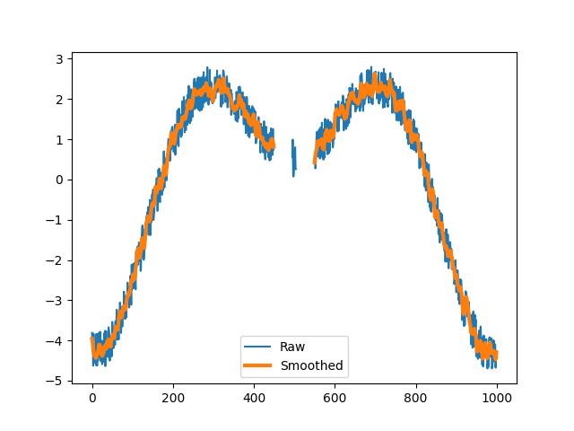
Apply the FIR lowpass filter with its default settings.

>>> xy_filt = fir_lowpass(xy)
>>> plt.plot(xy.x)
>>> plt.plot(xy_filt.x, linewidth=3)
>>> plt.legend(("Raw", "Smoothed"))
>>> plt.show()

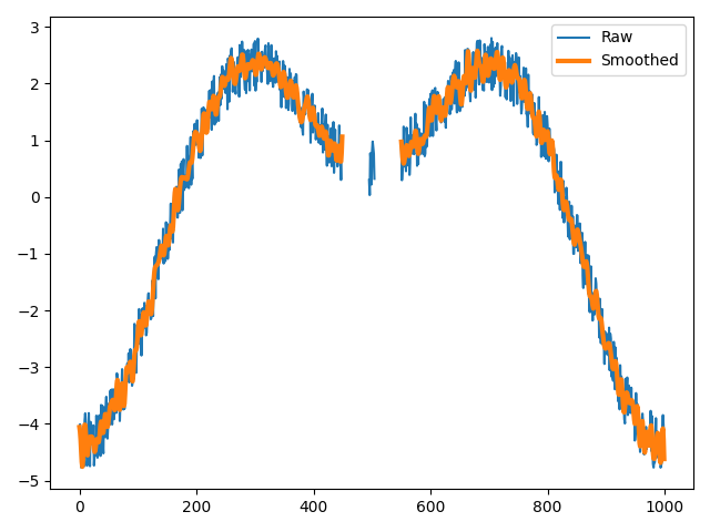
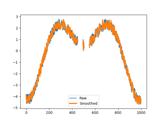
Apply the filter with different specifications.

>>> xy_filt = fir_lowpass(xy, numtaps=101, cutoff=3)
>>> plt.plot(xy.x)
>>> plt.plot(xy_filt.x, linewidth=3)
>>> plt.legend(("Raw", "Smoothed"))
>>> plt.show()

floodlight.transforms.filter.kalman(xy, process_noise=1.0, measurement_noise=0.04)

Applies a forward Kalman filter to an XY data object. [3]

Uses a constant-velocity motion model where the state vector consists of position and velocity. Only positions are observed. The filter smooths noisy position data by combining predictions from the motion model with the observed measurements.

Parameters:

• xy (XY) – Floodlight XY Data object. Must have framerate set.

• process_noise (float, optional) – Process noise intensity (acceleration variance in m²/s⁴) that controls how much the model trusts the constant-velocity prediction. Larger values allow faster changes in velocity. Default corresponds to \(\sigma_a = 1\,\mathrm{m/s^2}\), which is a conservative smoothing prior.

• measurement_noise (float, optional) – Measurement noise variance (in m²) controlling how much the model trusts the observed positions. Larger values produce smoother output. Default is 0.04, corresponding to 0.20 m RMSE, a conservative estimate for common optical [4] and local [5] tracking systems during high-dynamic situations.

Returns:

xy_filtered – XY object with position data filtered by the Kalman filter.

Return type:

XY

Notes

The Kalman filter requires xy.framerate to be set in order to compute the time interval between frames.

The default noise parameters assume positions are given in meters. If positions use a different unit (e.g. centimeters), the noise parameters must be adjusted accordingly (e.g. measurement_noise = 20.0**2 for 20 cm RMSE in centimeter units).

Unlike butterworth_lowpass() and savgol_lowpass(), the Kalman filter handles missing data (NaN) natively. When an observation is missing, the filter runs a predict-only step, maintaining its internal state (velocity estimate, covariance) across gaps. Frames with missing input data remain NaN in the output — no gap-filling is performed.

Examples

>>> import numpy as np
>>> import matplotlib.pyplot as plt
>>> from floodlight import XY
>>> from floodlight.transforms.filter import kalman

Generate a noisy XY-object to smooth.

>>> t = np.linspace(-5, 5, 1000)
>>> player_x = np.sin(t) * t + np.random.rand(1000)
>>> player_x[450:495] = np.nan
>>> player_x[505:550] = np.nan
>>> player_y = t + np.random.randn()
>>> xy = XY(np.transpose(np.stack((player_x, player_y))), framerate=20)

Apply the Kalman filter with default settings.

>>> xy_filt = kalman(xy)
>>> plt.plot(xy.x)
>>> plt.plot(xy_filt.x, linewidth=3)
>>> plt.legend(("Raw", "Smoothed"))
>>> plt.show()

Apply the filter with increased measurement noise for stronger smoothing.

>>> xy_filt = kalman(xy, measurement_noise=1.0)
>>> plt.plot(xy.x)
>>> plt.plot(xy_filt.x, linewidth=3)
>>> plt.legend(("Raw", "Smoothed"))
>>> plt.show()

References

[3]

Kalman, R. E. (1960). A New Approach to Linear Filtering and Prediction Problems. Journal of Basic Engineering, 82(1), 35-45.

[4]

Linke, D., Link, D., & Lames, M. (2020). Football-specific validity of TRACAB’s optical video tracking systems. PLoS ONE, 15(3), e0230179.

[5]

Blauberger, P., Marzilger, R., & Lames, M. (2021). Validation of player and ball tracking with a local positioning system. Sensors, 21(4), 1465.

floodlight.transforms.filter.savgol_lowpass(xy, window_length=5, poly_order=3, remove_short_seqs=False, **kwargs)

Applies a Savitzky-Golay lowpass-filter to an XY data object. [2]

For filtering, the scipy.filter.savgol function is used. This function provides a convenient access to the function, directly applying the filter to all non-NaN sequences in all columns.

Parameters:

• xy (XY) – Floodlight XY Data object.

• window_length (int, optional) – The length of the filter window. Corresponds to the argument window_length from the scipy.filter.savgol function. Default is 5.

• poly_order (Numeric, optional) – The order of the polynomial used to fit the samples. poly_order must be less than window_length. Default is 3. Corresponds to the argument poly_order from the scipy.filter.savgol function. Default is 5.

• remove_short_seqs (bool, optional) – If True, sequences that are too short for the filter with the specified settings are removed from the data. If False, they are kept unfiltered. Default is False.

• kwargs – Optional arguments {‘deriv’, ‘delta’, ‘mode’, ‘cval’} that can be passed to the scipy.signal.savgol function.

Returns:

xy_filtered – XY object with position data filtered by designed Savitzky-Golay low pass filter.

Return type:

XY

Notes

The values of the input data are assumed to be numerical. Missing data is assumed to be either np.nan or None. The Savitzky-Golay-filter requires a minimum signal length depending on the settings. A signal is a sequence of data in the XY-object that is not interrupted by missing values. The minimum signal length is defined as the window_length. The treatment of signals shorter than the minimum signal length are specified with the remove_short_sequence-argument, where True will replace these sequences with np.nan and False will keep the sequences in the data unfiltered.

Examples

>>> import numpy as np
>>> import matplotlib.pyplot as plt
>>> from floodlight import XY
>>> from floodlight.transforms.filter import savgol_lowpass

We first generate a noisy XY-object to smooth.

>>> t = np.linspace(-5, 5, 1000)
>>> player_x = np.sin(t) * t + np.random.rand(1000)
>>> player_x[450:495] = np.nan
>>> player_x[505:550] = np.nan
>>> player_y = t + np.random.randn()
>>> xy = XY(np.transpose(np.stack((player_x, player_y))), framerate=20)

Apply the Savgol lowpass filter with its default settings.

>>> xy_filt = savgol_lowpass(xy)
>>> plt.plot(xy.x)
>>> plt.plot(xy_filt.x, linewidth=3)
>>> plt.legend(("Raw", "Smoothed"))
>>> plt.show()

Apply the filter with a longer window length and remove the sequence that is too short to filter.

>>> xy_filt = savgol_lowpass(xy, window_length=12, remove_short_seqs=True)
>>> plt.plot(xy.x)
>>> plt.plot(xy_filt.x, linewidth=3)
>>> plt.legend(("Raw", "Smoothed"))
>>> plt.show()

Apply the filter with different specifications.

>>> xy_filt = savgol_lowpass(xy, window_length=50, poly_order=5)
>>> plt.plot(xy.x)
>>> plt.plot(xy_filt.x, linewidth=3)
>>> plt.legend(("Raw", "Smoothed"))
>>> plt.show()

References

[2]

Savitzky, A.; Golay, M.J. (1964). Smoothing and differentiation of data by simplified least squares procedures. Analytical Chemistry, 36(1), 1627- 1639.

floodlight.transforms.filter.wiener(xy, window_size=5, noise=None, remove_short_seqs=False)

Applies a Wiener filter to an XY data object. [6]

For filtering, the scipy.signal.wiener function is used. This function provides a convenient access to the function, directly applying the filter to all non-NaN sequences in all columns.

Parameters:

• xy (XY) – Floodlight XY Data object.

• window_size (int, optional) – Size of the local window used for noise estimation and filtering. Corresponds to the argument mysize from the scipy.signal.wiener function. Default is 5.

• noise (float, optional) – Noise power estimate. If None, the noise power is estimated locally from the data within the window. Corresponds to the argument noise from the scipy.signal.wiener function. Default is None.

• remove_short_seqs (bool, optional) – If True, sequences that are too short for the filter with the specified settings are replaced with np.nan. If False, they are kept unfiltered. Default is False.

Returns:

xy_filtered – XY object with position data filtered by the Wiener filter.

Return type:

XY

Notes

The values of the input data are assumed to be numerical. Missing data is assumed to be either np.nan or None. The Wiener filter requires a minimum signal length depending on the settings. A signal is a sequence of data in the XY-object that is not interrupted by missing values. The minimum signal length is defined as the window_size. The treatment of signals shorter than the minimum signal length are specified with the remove_short_seqs-argument, where True will replace these sequences with np.nan and False will keep the sequences in the data unfiltered.

Examples

>>> import numpy as np
>>> import matplotlib.pyplot as plt
>>> from floodlight import XY
>>> from floodlight.transforms.filter import wiener

We first generate a noisy XY-object to smooth.

>>> t = np.linspace(-5, 5, 1000)
>>> player_x = np.sin(t) * t + np.random.rand(1000)
>>> player_x[450:495] = np.nan
>>> player_x[505:550] = np.nan
>>> player_y = t + np.random.randn()
>>> xy = XY(np.transpose(np.stack((player_x, player_y))), framerate=20)

Apply the Wiener filter with its default settings.

>>> xy_filt = wiener(xy)
>>> plt.plot(xy.x)
>>> plt.plot(xy_filt.x, linewidth=3)
>>> plt.legend(("Raw", "Smoothed"))
>>> plt.show()

Apply the filter with a larger window size for stronger smoothing.

>>> xy_filt = wiener(xy, window_size=25)
>>> plt.plot(xy.x)
>>> plt.plot(xy_filt.x, linewidth=3)
>>> plt.legend(("Raw", "Smoothed"))
>>> plt.show()

References

[6]

Wiener, N. (1949). Extrapolation, Interpolation, and Smoothing of Stationary Time Series. MIT Press.